
Predicting Teleworking Issues With Machine Learning
The goal of this experiment is to predict and classify network issues that teleworkers may experience whilst working from home. It will be achieved by analyzing network performance and configuration data collected from each computer using machine learning technology. I won’t go into details about how the data is collected, that’s a seperate subject. The machine learning prediction will classify issues such as Wi-Fi, wired LAN, Internet or None (in case there is no issue detected).
The method of machine learning model that will be applied is known as multi-class classification, meaning it predicts one class (label) from a series of three or more discrete classes. Other types of model include binary (two classes), or regression (numberical prediction).
I selected to use Google AutoML because it is very quick and simple to get started.
Data Features
Machine Learning requires ‘Features’ to build the model; these are the values used to determine the prediction. The dataset includes the following features for each computer:
- Latency to corporate network test page (10th percentile - last 24hrs)
- Latency to corporate network test page (90th percentile - last 24hrs)
- Latency to Internet test page (10th percentile - last 24hrs)
- Latency to Internet test page (90th percentile - last 24hrs)
- Latency to LAN gateway (10th percentile - last 24hrs)
- Latency to LAN gateway (90th percentile - last 24hrs)
- Wi-Fi Channel Number
- Wi-Fi Signal Strength Percentage (average - last 24hrs)
- VPN gateway name
- Issue (None, LAN, WiFi, Internet)
Data Preperation
This is the most important and time-consuming part of the process. I created a SQL database query to retrieve the data in a structure where there is a row for each computer, with columns for each feature (listed above). I then manually provided the target data (answers) for the ‘Issue’ column which will be used for training. For supervised machine learning you must provide the ‘correct answers’ in the training data. The more data you provide, the more accurate the model will be.
The minimum number of rows required is 1,000 for Google AutoML. The more features you add, the more training data you should provide. Below is a sample of the training data, note that the ‘Issue’ column on the far right has been populated by myself. The training data set contains information about 1,600 computers.
Here’s a sample of the data. Highlighted in yellow are some indicators of network performance issues:
| percentile_10_corporate | percentile_90_corporate | percentile_10_internet | percentile_90_internet | percentile_10_lan | percentile_90_lan | wlan_signal | wlan_in_use | wlan_channel | vpn_gateway | issue |
|---|---|---|---|---|---|---|---|---|---|---|
| 62 | 102 | 202 | 2165 | 24 | 344 | 49 | TRUE | 6 | location1 | wifi |
| 183 | 2967 | 355 | 2592 | 0 | 5 | 99 | TRUE | 6 | location1 | internet |
| 277 | 311 | 585 | 455 | 1 | 171 | 83 | TRUE | 36 | location4 | none |
| 103 | 138 | 196 | 308 | 16 | 229 | 93 | FALSE | 4 | location6 | lan |
| 170 | 409 | 353 | 1018 | 1 | 11 | 0 | FALSE | 0 | location8 | internet |
| 225 | 384 | 466 | 219 | 1 | 15 | 77 | TRUE | 6 | location10 | none |
| 228 | 303 | 472 | 488 | 1 | 4 | 99 | TRUE | 11 | location1 | none |
| 200 | 211 | 430 | 456 | 2 | 64 | 78 | TRUE | 6 | location14 | none |
Import the training data
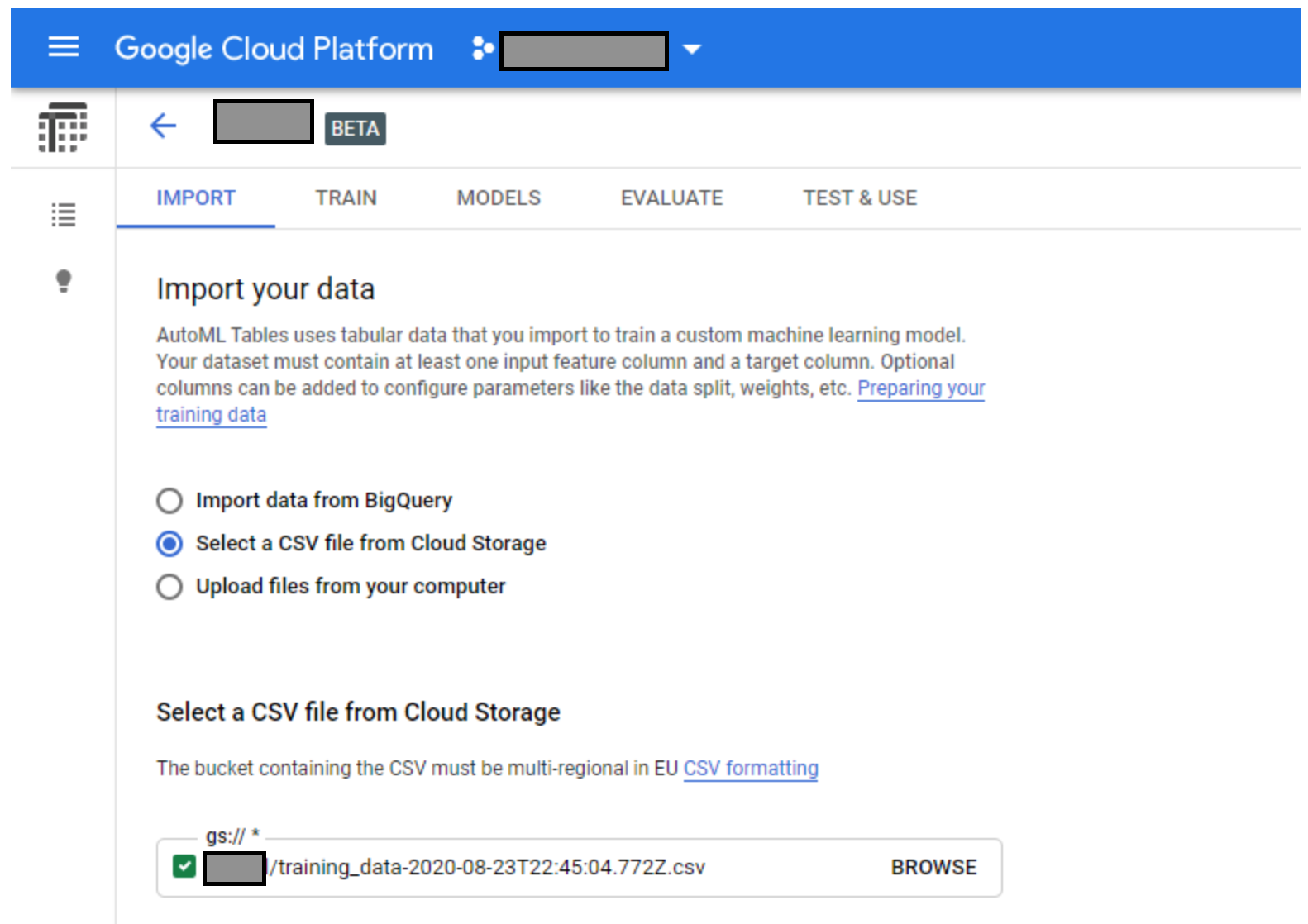
Once the training data is ready it can be uploaded directly (in CSV format) from your computer, or imported from a Google Cloud storage bucket. Alternatively, you can provide the data in a BigQuery database table.
Screenshot showing import of data from Google storage bucket
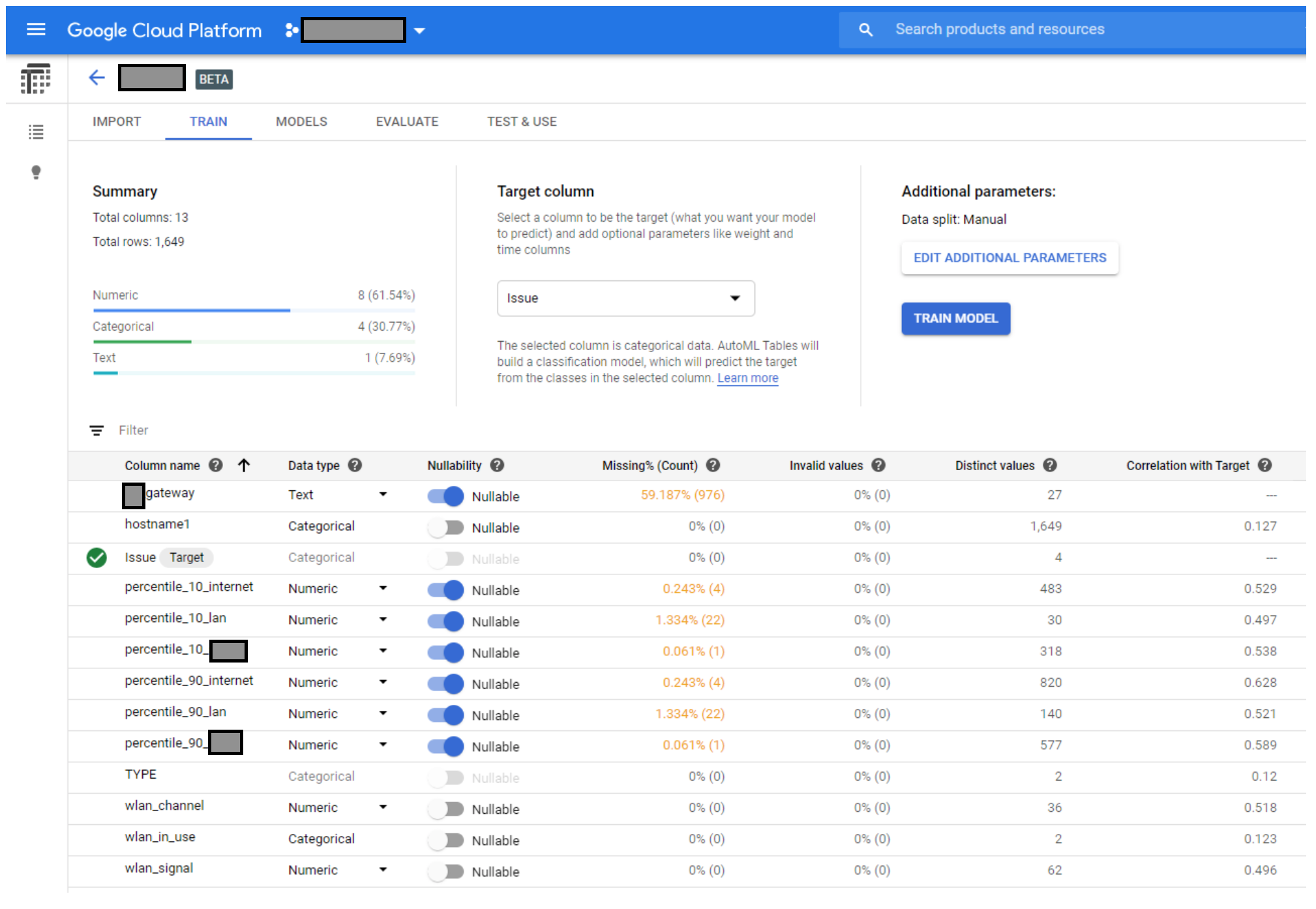
Configure the training the model
AutoML uses supervised training (example data with known results) to improve accuracy. As ML performs training it verifies the outcome of the predictions against the validation (10%) data. The precision (accuracy) of the machine learning is determined by using the remaining test (10%) data.
Screenshot showing data training settings
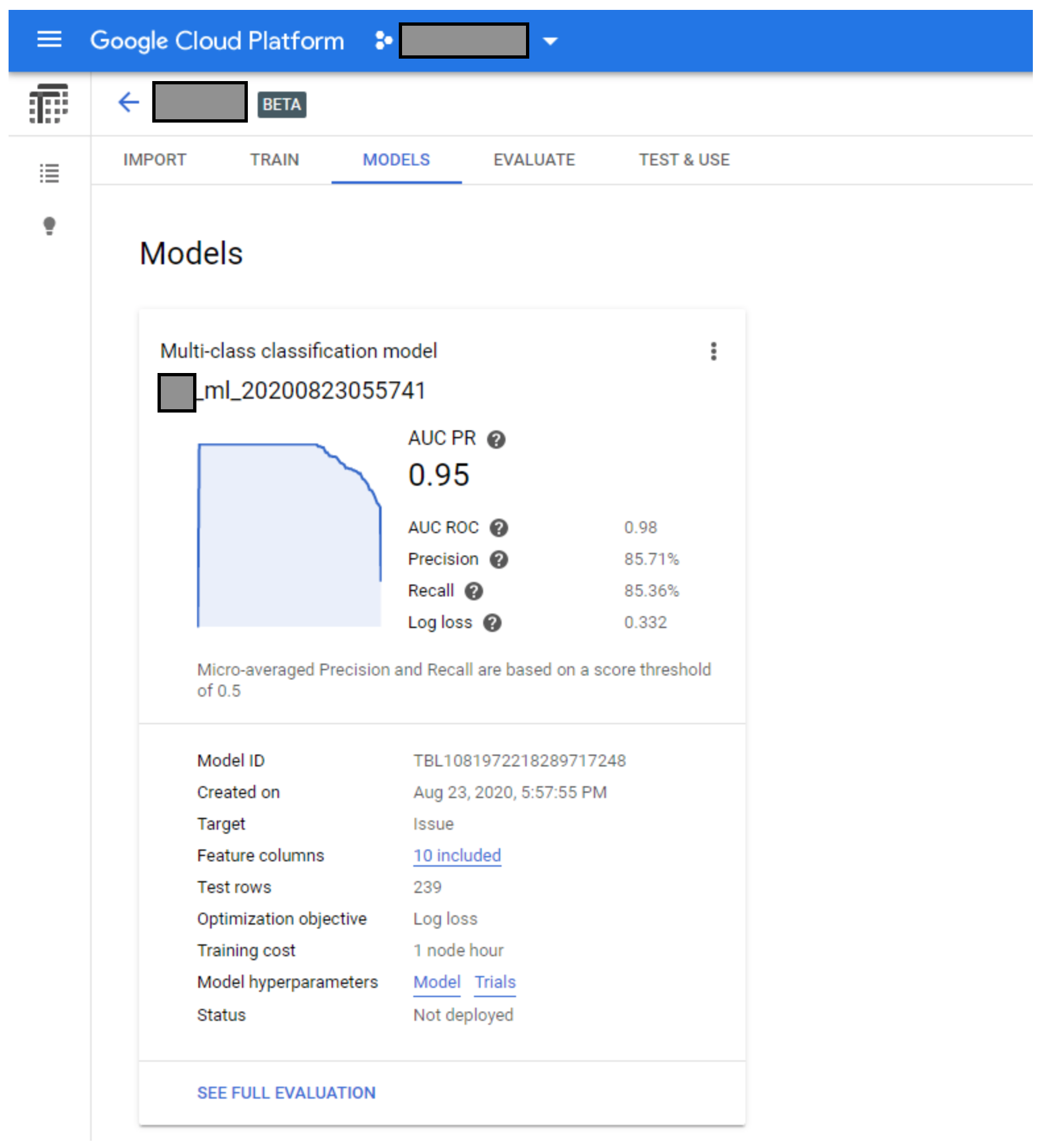
Evaluate the training results
Once the training completes you can evaluate how accurate the model is. Precision incidates the percentage of tests where machine learning successfully identified the correct classification for the test (10%) portion of the training dataset.
Using the sample network performance data I uploaded, the outcome of ML training was 86% precision. This means 86% of the time ML successfully predicted the classification (Issue) and exactly matched the known test data.
Screenshot showing results of training
Utilize the machine learning model
Now that the machine learning model has been created, we have three options to use it:
- Batch Prediction - manual, providing data in CSV format or BigQuery table
- Online Prediction - creates a API endpoint hosted in Google Cloud
- Export Model - download the model as a TensorFlow package for local use
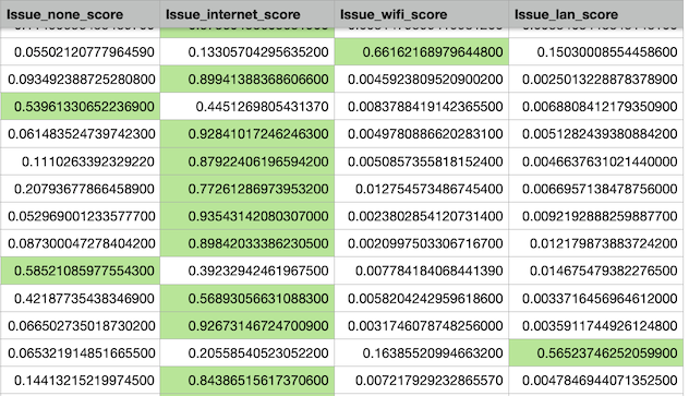
For this experiment I used batch prediction and uploaded data for 5,000 computers for which I didn’t know the ‘Issue’ and ran the data through the ML model. After downloading the results new columns were available, one for each category (None, Wi-Fi, LAN and Internet).
For each computer/row, and for each classification (Issue) there is a score with the probability. The batch took four minutes to execute.
Highlighted in green is the category (Issue) which had the highest probability. As we know from the training data, the accuracy should be around 86%
Analysis of Internet versus LAN latency
I knew from the results of the machine learning that the Internet and LAN latency 90th percentile features were the most important factors. To check if the machine learning results made sense I decided to create a scatter graph and compare the two most important features.
import plotly.express as px
import plotly.offline as pyo

pyo.init_notebook_mode()

# create a scatter graph with 90pc latency for LAN versus Internet
fig = px.scatter(
    df.query('percentile_90_internet < 4000 & percentile_90_lan <4000'),
    x="percentile_90_internet", y="percentile_90_lan",
    title="Internet versus LAN latency by Issue",
    color="Issue",
    labels = {
        'percentile_90_internet': 'Internet Latency (MS)',
        'percentile_90_lan': 'LAN Gateway Latency (MS)',
        }
    )
# display graph
fig.show()
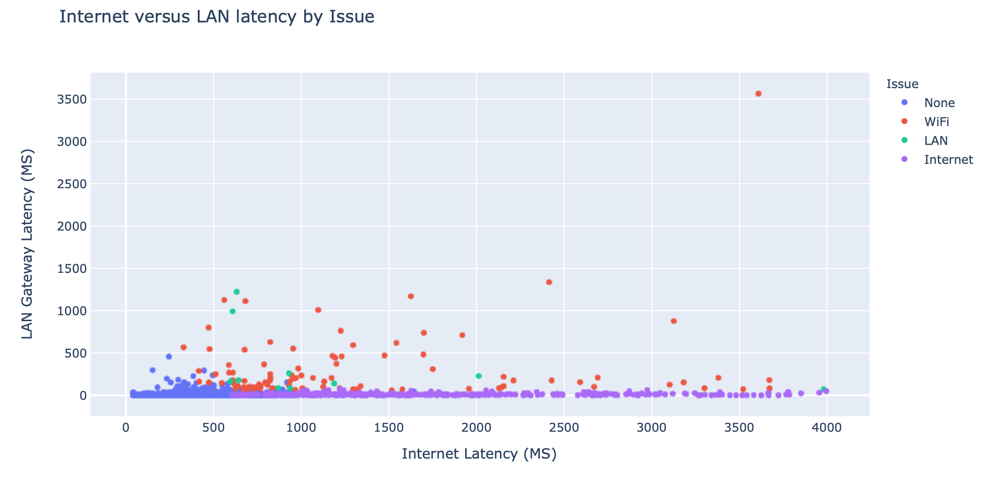
From the chart I was able to validate that:
- When both LAN and Internet latency are low no issue is detected
- When Internet latency is high, but LAN is low the issue is Internet (as expected)
- When LAN latency is high the issue is LAN or Wi-Fi (I infer that if LAN issues would cause Internet to be poor too)
Analysis of Wi-Fi signal strength versus channel number
The local network is under the control of the teleworker; it’s the component of the network that they can have the most influence over. I was curious to see what they could do to improve their connectivity. I expected there to be a correlation between poor LAN performance and Wi-Fi signal strength/channel.
# create a scatter graph with Wi-Fi channel versus signal strength
fig = px.scatter(
    df.query('Issue != "Internet" and Issue != "LAN"'),
    x="wlan_channel",
    y="wlan_signal",
    title="Wi-Fi Signal versus Channel by Issue (excluding Internet)",
    color="Issue",
    labels = {
        'wlan_signal': 'Wi-Fi Signal Strength (%)',
        'wlan_channel': 'Wi-Fi Channel Number',
        }
    )
# display graph
fig.show()
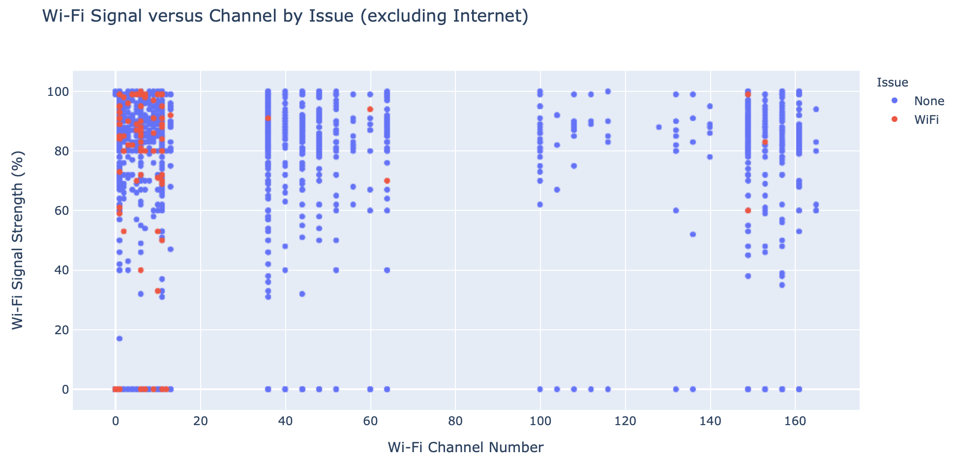
I found that the majority of Wi-Fi issues occur on 2.4Ghz channels, which is expected. Interestingly, many issues affect 2.4Ghz users with good signal strength. This indicates that high LAN latency could be caused by interference. I can also conclude that for those users with strong Wi-Fi signal strength it would be safe to advise switching to 5Ghz which is often less congested.
Conclusion
At the end of this experiment I’m happy with the progress I made, given minimal time investment. It was a fun project to try machine learning for the first time. Google AutoML makes it incredibly easy to get started, and accuracy of 86% is pretty good!.
I’d like to find a way to generate training data automatically, and also provide feedback to the machine learning model for continous improvement. Machine learning will become more important as the dataset grows and more features are added which require analysis.