Optimising Grafana Visualization for Vertica Databases

Recently I’ve been using Grafana to visualise time series data from a Vertica Database. This article covers some of the techniques I found to optimise the performance of SQL queries/visualization.

Grafana

Grafana is an open-source observability platform, supporting a vast range of data sources, including Vertica. It’s highly extensible via a plug-in ecosystem, supporting many different types of data including metrics, logs, and traces. Dashboards are built from modular panels, with a variety of different charts/visualizations available.

Documentation for the Vertica data source includes the supported built-in variables which are required to optimise data queries.

There is also a really nice demo website (https://play.grafana.org/) where you can explore Grafana and its functionality.

Vertica

Vertica is a high performance relational, analytical database from OpenText, designed to handle extremely large datasets. It uses a columnar storage architecture, and makes significant use of compression to reduce storage, and increase data retention. To explore a Vertica database I recommend DBeaver, an open-source (Apache License) database client which supports many different types of database connections.

Use Case

In this example I’m using a database which is part of OpenText Network Operations Management (NOM) OPTIC solution, which collects and stores network device resource metrics. I’ll create charts to visualise interface utilization, as well as error and discard rates.

OpenText NOM provides three tables with different levels of data aggregation for interface metrics, these are 5-Minute, Hourly, and Daily.

Complete SQL Query

Below is the complete SQL query for reference.

SELECT 
  descr.node_short_name || ' - ' || descr.netif_description || ' (' || LEFT(descr.netif_alias, 40) || ')' AS ifname, 
  sq.throughput_in AS BW_In, 
  sq.throughput_out AS BW_Out, 
  sq.discards_out, 
  sq.errors_in, 
  sq.ts 
FROM 
  (
    SELECT 
      netif_qname AS ifName, 
      netif_unique_id, 
      TIME_SLICE(
        to_timestamp(timestamp_utc_s), 
        $__interval_ms, 
        'MILLISECOND'
      ) AS ts, 
      AVG(throughput_in_mbit_per_s) AS throughput_in, 
      AVG(throughput_out_mbit_per_s) AS throughput_out, 
      AVG(discard_out_pct) AS discards_out, 
      AVG(error_in_pct) AS errors_in 
    FROM 
      mf_shared_provider_default.nom_interface_health a 
    WHERE 
      '$__interval' LIKE '%m%' 
      AND $__unixEpochFilter(timestamp_utc_s) 
      AND node_unique_id IN (${device}) 
      AND netif_unique_id IN (${interface}) 
    GROUP BY 
      ts, 
      ifName, 
      netif_unique_id 

    UNION ALL

    SELECT 
      netif_qname AS ifName, 
      netif_unique_id, 
      TIME_SLICE(
        to_timestamp(timestamp_utc_s), 
        $__interval_ms, 
        'MILLISECOND'
      ) AS ts, 
      AVG(throughput_in_avg_mbit_per_s) AS throughput_in, 
      AVG(throughput_out_avg_mbit_per_s) AS throughput_out, 
      AVG(discard_out_avg_pct) AS discards_out, 
      AVG(error_in_avg_pct) AS errors_in 
    FROM 
      mf_shared_provider_default.nom_interface_health_1h b 
    WHERE 
      '$__interval' LIKE '%h%' 
      AND $__unixEpochFilter(timestamp_utc_s) 
      AND node_unique_id IN (${device})
      AND netif_unique_id IN (${interface}) 
    GROUP BY 
      ts, 
      ifName, 
      netif_unique_id

    UNION ALL
  
    SELECT 
      netif_qname AS ifName, 
      netif_unique_id, 
      TIME_SLICE(
        to_timestamp(timestamp_utc_s), 
        $__interval_ms, 
        'MILLISECOND'
      ) AS ts, 
      AVG(throughput_in_avg_mbit_per_s) AS throughput_in, 
      AVG(throughput_out_avg_mbit_per_s) AS throughput_out, 
      AVG(discard_out_avg_pct) AS discards_out, 
      AVG(error_in_avg_pct) AS errors_in 
    FROM 
      mf_shared_provider_default.nom_interface_health_1d 
    WHERE 
      '$__interval' LIKE '%d%' 
      AND $__unixEpochFilter(timestamp_utc_s) 
      AND node_unique_id IN (${device}) 
      AND netif_unique_id IN (${interface}) 
    GROUP BY 
      ts, 
      ifName, 
      netif_unique_id
  ) AS sq 

  LEFT OUTER JOIN (
    SELECT 
      ISNULL(netif_alias, '-') AS netif_alias, 
      ISNULL(netif_description, '-') AS netif_description, 
      netif_unique_id, 
      node_short_name 
    FROM 
      mf_shared_provider_default.nom_entity_interface_raw
  ) AS descr ON sq.netif_unique_id = descr.netif_unique_id 
GROUP BY 
  ts, 
  ifname, 
  netif_alias, 
  node_short_name, 
  sq.throughput_in, 
  sq.throughput_out, 
  sq.discards_out, 
  sq.errors_in, 
  netif_description 
ORDER BY 
  TS

Timeslice

The Vertica Time_Slice function aggregates data by the specified time interval.

Grafana supports the ability to use dynamic time intervals, automatically calculated based on the time window selected by the user (e.g. last 7 days), the width of the chart (pixels), and optionally, maximum desired data points.

The calculated time interval is provided via the $__interval (e.g. 15m) and $__interval_ms (e.g. 900000ms) variables.

Passing in the $__interval_ms variable, and setting the time unit to Milliseconds ensures accurate aggregation.

TIME_SLICE(to_timestamp(timestamp_utc_s), $__interval_ms, 'MILLISECOND')

Selecting the appropriate table

Querying the 5-Minute table for 30 days worth of data is clearly not efficient, given the thousands of rows of data that would need to be processed. For longer time windows we need a mechanism to use the hourly or daily aggregation tables instead.

To achieve this logic I took advantage of the Grafana $__interval variable which indicates resolution of ‘m’, ‘h’ and ‘d’ (e.g. ‘15m’ for 15 minutes). I can match these using a where clause to return data from the appropriate table.

The logic is essentially to merge multiple select statements for each table, however only one of the tables will return any data matching the appropriate aggregation (minutes, hours, days):

Pseudo code for combining multiple select statements with conditions

SELECT FROM (
  SELECT
  -- 5-min table
  FROM table_5_min_aggregation
  WHERE $__interval like '%m%' 

  UNION ALL

  SELECT
  -- Hourly table
  FROM table_hourly_aggregation
  WHERE $__interval like '%h%'

  UNION ALL

  SELECT
  -- Daily table
  FROM table_daily_aggregation
  WHERE $__interval like '%d%'
)

Grafana Max Data Points

Grafana automatic time interval calculation is a fantastic feature because it enables appropriate scaling of the data/query based on the time window selected by the user, however by default I found the visual appearance of the graph to be quite unappealing with far too many data points shown, also queries took an excessive time to load.

By setting the maximum data points it helped to select a visually appealing time interval, and improved performance quite dramatically.

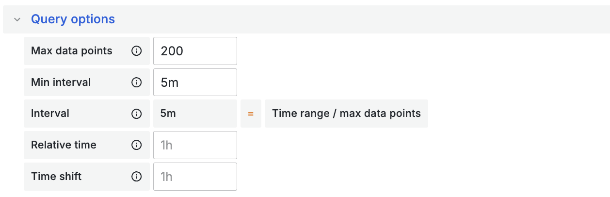
Chart for 7-day period, with 1,661 data points (automatically calculated) at 5-minute interval - it took 14.4 seconds to load, all data came from the 5-Minute table.

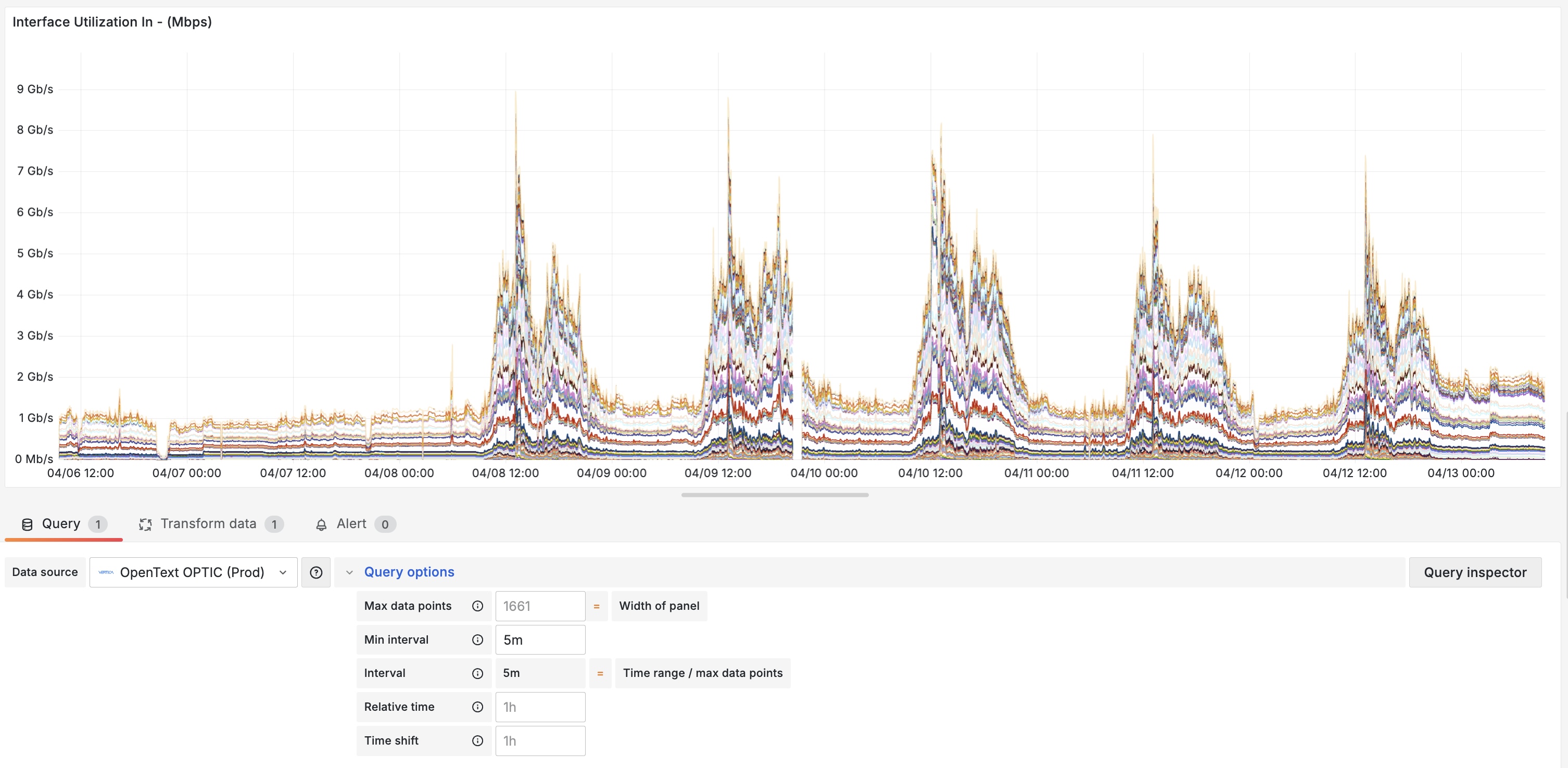
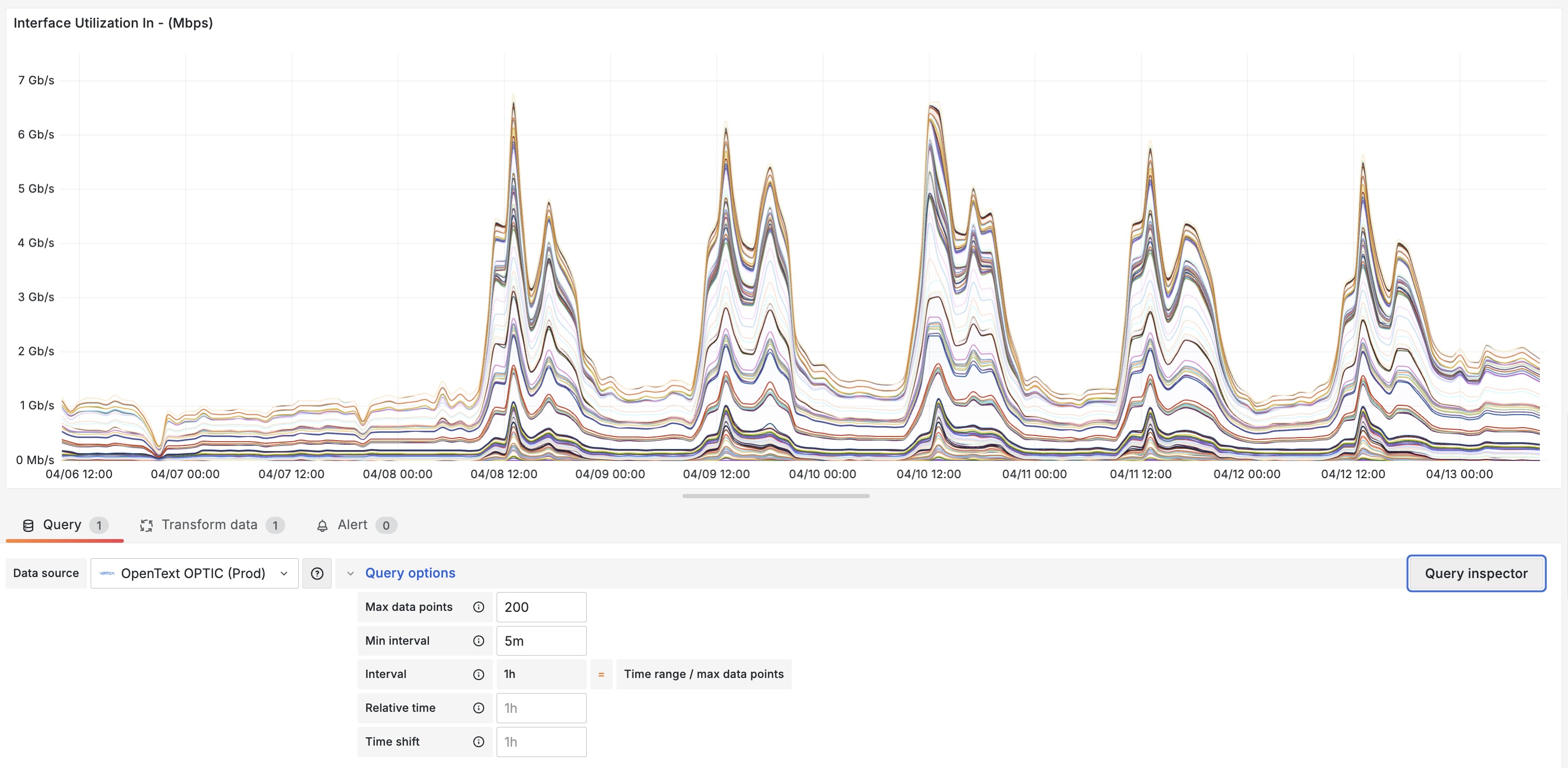
Chart for same time period, but with 200 (fixed) data points (now calculated at 1-hour interval) - taking 2.4 seconds to load, with all data coming from the hourly table. Visual appearance has also improved.

Grafana Query Re-Use

A nice feature of Grafana is the ability to create multiple charts with a single database query. Typically it’s more efficient to make one query for four metrics, than to make four queries each with a single metric.

After creating the first query/visualization (with multiple metrics selected), create the next visualization and choose the data source ‘Dashboard’, and select the panel created previously.

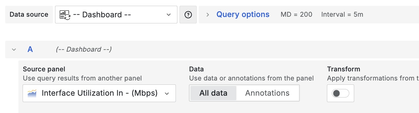
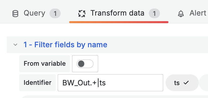
At this point, you’ll see each panel has the same/many metrics shown; to show only the relevant metrics in each chart, apply the transformation ‘Filter fields by name’. In this case I only need the Timestamp (ts), and ‘BW_Out*’ metrics.

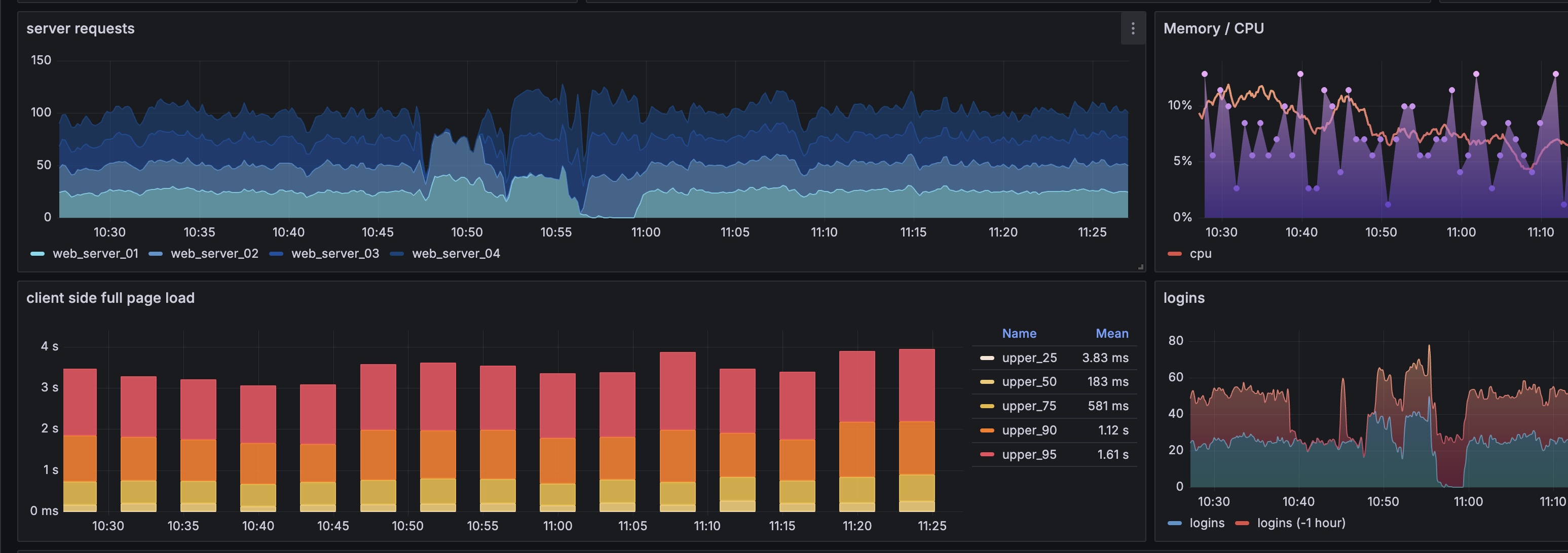
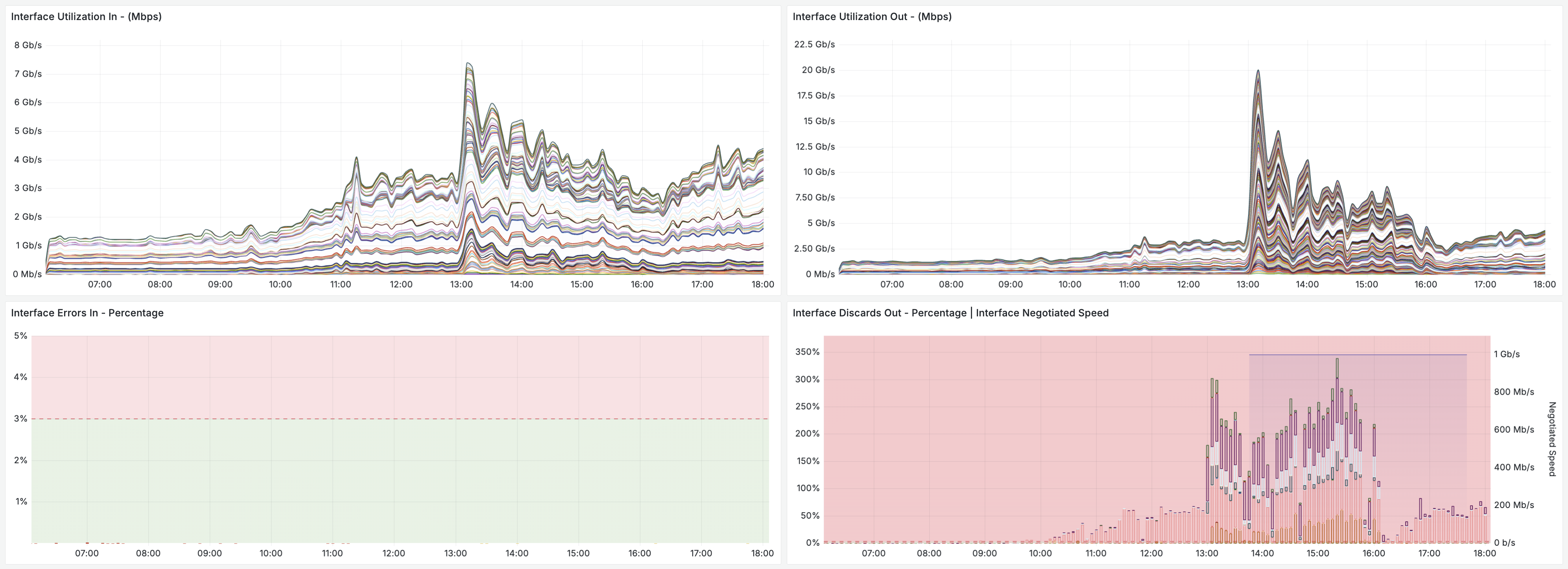
Screenshot showing four charts using data from a single query, improving time to load by 70% or more.

Wrap-Up

This was my first experience using a Vertica data source with Grafana, after iterating/discovering these optimizations I was able to successfully improve the performance of the dashboard quite considerably, from 15 seconds to around 2-3 seconds.

If you have any suggestions please let me know!